Many modern 2D renderers convert Bézier curves into polylines in order to render them. This results in a simpler painting algorithm since it only has to know how to render one single type of primitive: a line.

Given some initial tolerance, the question of how to split a Bézier into lines is fairly involved. I'd argue that there are two traditional answers:

1. Recursively subdividing the curve until each section is flat enough that it can be replaced with a line, according to the tolerance.
2. Finding, in parametrized space (e.g. curve's t), the largest section that falls within the tolerance, then dividing the parametrized space equally such that all sections are smaller or equal to that section.

The first approach cannot be parallelized, but results in a number of lines decently close to the ideal. The second can be parallelized, but it generates too many lines in places where the curve is rather flat.

In a modern renderer, both of these properties are desirable. The low number of lines enables the curves to be cached in a compact, memory-efficient form that can still be manipulated as long as it is not scaled up. The second property, parallelization, is hopefully self-evident.

An elegant way to eliminate this trade-off is by using Raph Levien's analytic quadratic Bézier flattener which is also fully parallelizable. Since forma needs a good solution for stroked paths, I decided to extend his method to quadratic curve offsets. Because forma lowers cubic Béziers to quadratics in the first place, this method would be sufficient for all stroking needs.

The closest approach to this is described by Fabian Yzerman where all curves are approximated by quadratics which is then followed by a curvature-aware, iterative approach. This provides something closer to a fully analytical method, but is limited by the data-dependency that keeps it from having parallelization potential.

In the end, I started from Raph's formula (which applies to the \(x ^ 2\) parabola), where \(l\) is the arc length and \(\kappa\) is the curvature:

$$ segments = \frac{q}{2 \sqrt{2}} \int_{x_0}^{x_1} l(x)\sqrt{\kappa(x)} dx, $$

$$ \quad q = \sqrt{\frac{scale}{tolerance}} $$

The interesting part of the formula above is the integral which is virtually the point density of the curve from \(x_0\) to \(x_1\):

$$ \rho(x_0, x_1) = \int_{x_0}^{x_1} l(x)\sqrt{\kappa(x)} dx $$

This can then be extended to a version that takes the distance \(d\) to the curve:

$$ \rho(x_0, x_1, d) = \int_{x_0}^{x_1} l(x, d)\sqrt{\kappa(x, d)} dx $$

Taking advantage of a curve offset property, curvature is:

$$ \kappa(x, d) = \frac{\kappa(x)}{1 + d \kappa(x)} $$

For the parabola parallel curve arc length and curvature end up:

$$ l(x, d) = \sqrt{x ^ 2 \left(\frac{4 d}{\left(4 x ^ 2 + 1\right) ^ {\frac{3}{2}}} + 2\right) ^ 2 + 1} $$

$$ \kappa(x, d) = \frac{1}{d + \frac{1}{2} \left(4 x ^ 2 + 1\right) ^ {\frac{3}{2}}} $$

Unsurprisingly, I couldn't find any analytical solution to \(\rho \) and especially \(\rho ^ {-1} \). A solution to the integral with an infinite sum/fraction may be possible, but finding an inverse would be significantly more challenging.

I saw two possible ways forward to approximate these two functions.

Symbolic regression

Symbolic regression is a method of finding pure mathematical approximations to a set of points of dimension 2+. A good starting point would be SRBench, specifically the black-box section in the results page.

From that list, I tried Operon, MRGP, and DSR, with Operon giving the best results. The error from the most accurate solution varied from 0.05% all the way to a few thousand % for small values of \(x\) and \(d\).

Weighting the points might have resulted in better overall accuracy, but I ended up abandoning this path since no symbolic regressor seemed to have the ability to scale: regardless of the amount of time/space used, or how large the ensuing output was, it never seemed to come close to the accuracy that was needed here.

Nonetheless, I still think symbolic regression might be something worth revisiting when solvers become more robust and manage to scale with time and complexity.

Interpolation

Suffice to say that interpolation was a significant improvement in terms of accuracy. I used SciPy's interpolation library which, in turn, uses DIERCKX. This generates a 2D B-spline that's decently cheap to evaluate.

The key to good accuracy in this case is finding interesting points for the grid. I simply picked these points manually in order to minimize the error against the goal surface. This worked well in practice and, with an optimized implementation in Rust, it seems to have satisfactory performance.

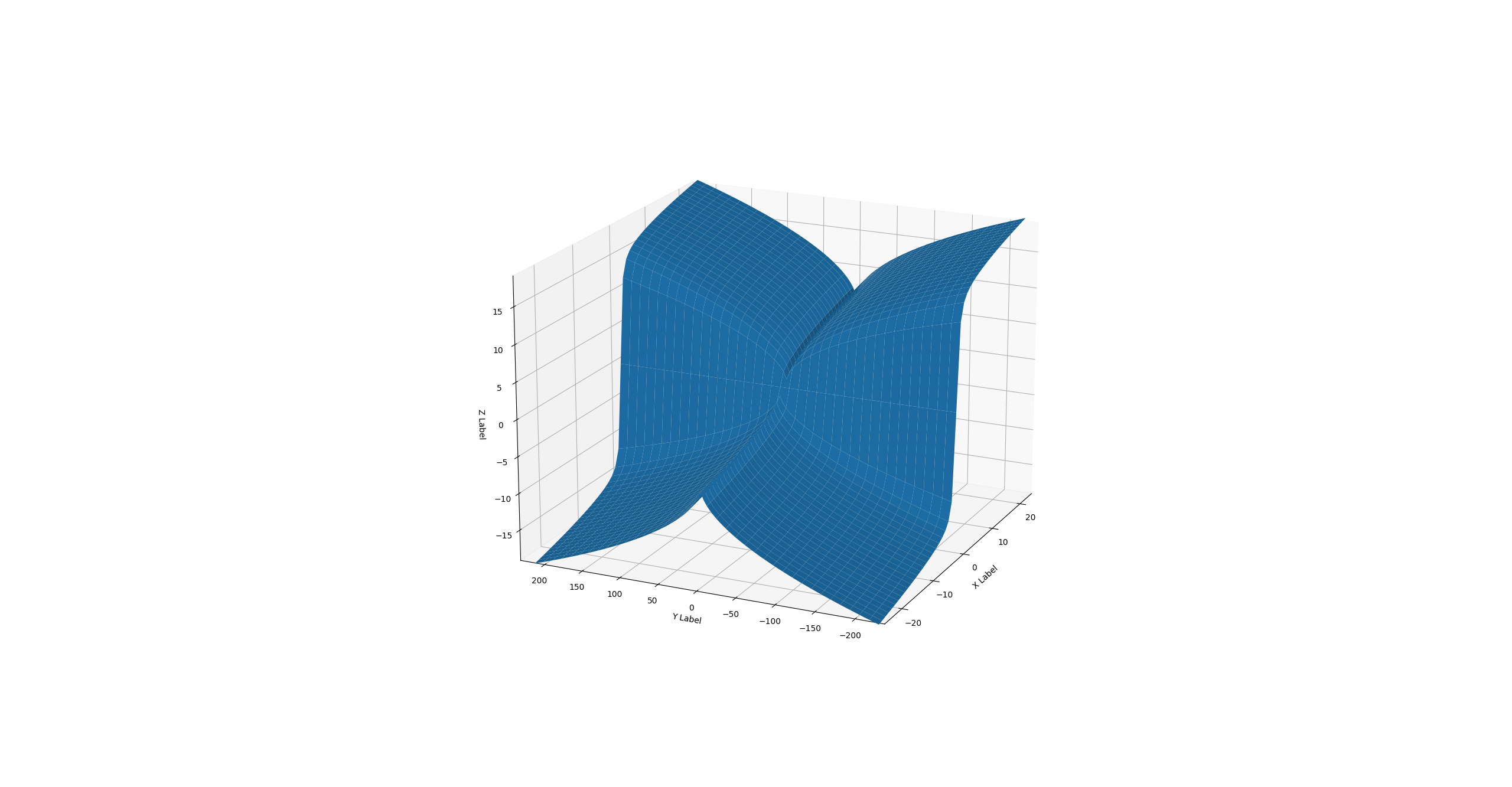
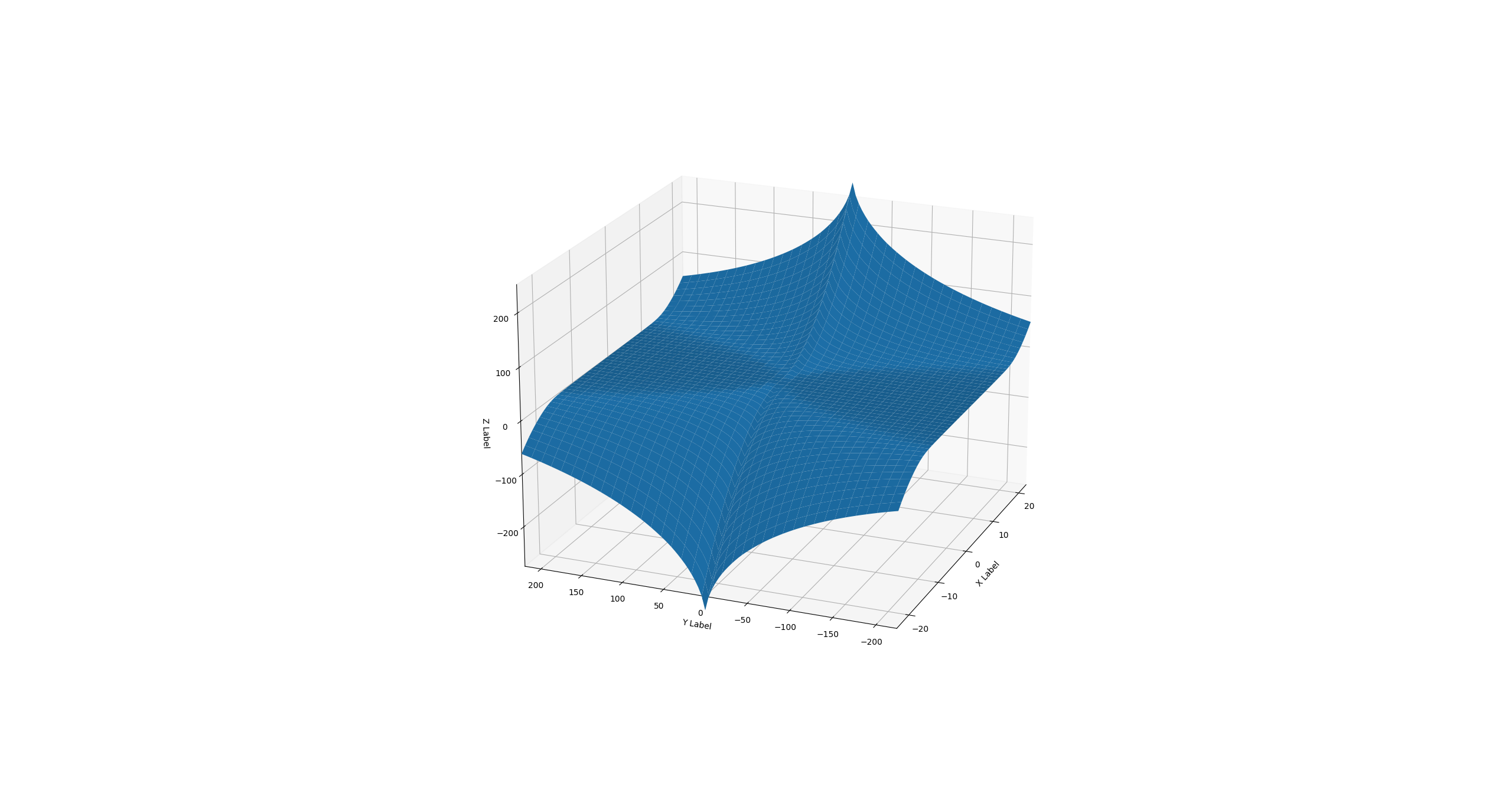
The following are the density and the inverse approximated by B-splines:

Future work

Improvement is likely be possible by either finding a pure approximation (maybe with symbolic regression) or by finding an alternative interpolation that evaluates even faster than the 2D B-spline.

Demo in egui

The demo below showcases the approach using B-splines to approximate the two functions. The code will be made available on GitHub once the implementation reaches maturity in terms of stability and efficiency.